Plots

metafopy draws plots with matplotlib. Each plot function draws on the current axes (or on an axes object passed as ax=) and returns a result object that holds what was plotted. Save and show figures with the usual matplotlib functions.

The plot gallery reproduces the plots of the metafor documentation with metafopy, and compares them with the R figures.

import matplotlib

matplotlib.use('Agg')

import matplotlib.pyplot
import numpy

from metafopy import datasets, escalc, rma

dat = escalc(measure='RR', ai='tpos', bi='tneg', ci='cpos', di='cneg', data=datasets.load('dat.bcg'))
dat['label'] = dat['author'] + ', ' + dat['year'].astype(str)
res = rma('yi', 'vi', data=dat, slab=dat['label'])

Forest plot

from metafopy import forest

forest(res, atransf=numpy.exp, header=True)
matplotlib.pyplot.savefig('forest.png', dpi=150)

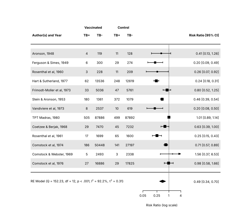
atransf transforms the axis labels (here to risk ratios) while the plot stays on the log scale, and transf transforms the estimates themselves. Other common arguments are:

• order: 'obs' sorts by effect size, 'prec' by precision, or give your own values.
• ilab, ilab_lab, ilab_xpos: columns of study information shown next to the plot.
• addpred=True: add the prediction interval to the summary.
• showweights=True: show the weights.
• xlim, alim, at, refline, xlab, digits, slab.
• na_action='pass': keep the studies dropped for missing values as (empty) rows of the plot, as metafor does under options(na.action='na.pass').

For plots with subgroups, draw the studies with forest(..., rows=...) and the summaries with addpoly. Examples are in the metafor documentation: https://www.metafor-project.org/doku.php/plots:forest_plot_with_subgroups. The gallery also reproduces the BMJ, RevMan and superscript styles.

from metafopy import forest

forest(res, atransf=numpy.exp, order='obs', addpred=True, xlab='Risk ratio')
matplotlib.pyplot.savefig('forest-sorted.png')

Funnel plot

from metafopy import funnel

matplotlib.pyplot.figure()
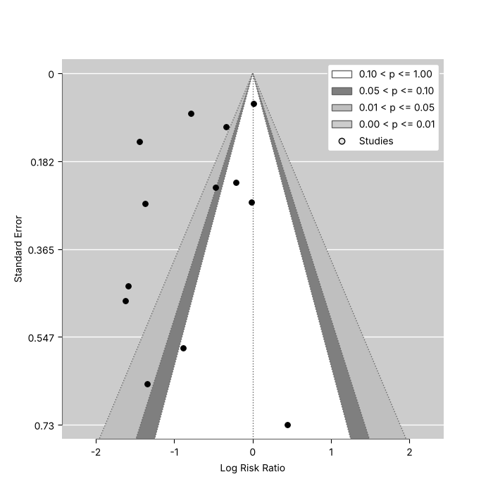
funnel(res)
matplotlib.pyplot.savefig('funnel.png')

yaxis sets the vertical axis ('sei' is the default, also 'vi', 'seinv', 'vinv', 'ni', 'ninv', 'sqrtni', 'sqrtninv', 'lni', 'wi'), level and shade draw the contours of statistical significance (contour-enhanced funnel plots, Peters et al., 2008, https://doi.org/10.1016/j.jclinepi.2007.11.010), and funnel(trimfill(res)) shows the filled studies.

matplotlib.pyplot.figure()
funnel(res, level=[90, 95, 99], shade=['white', 'gray55', 'gray75'], refline=0)
matplotlib.pyplot.savefig('funnel-contours.png')

Other plots

Function	Plot
radial	Radial (Galbraith) plot
labbe	L'Abbe plot of 2x2 table event rates
baujat	Baujat plot, which studies drive the heterogeneity
qqnorm	Normal quantile-quantile plot of the residuals, with a simulated envelope
plot_infl	Case deletion diagnostics, see Diagnostics
plot_profile	Profile likelihood of a variance component, from profile; given the list profile returns for rma_mv, location-scale and selection models it draws one panel per component
plot_gosh	GOSH plot
regplot, points_regplot	Meta-analytic scatterplot of a model with one moderator (rma_uni, location-scale, selmodel, rma_mv and rma_glmm fits), with the regression line, confidence band and sized points; points_regplot redraws the points and labels of the result
forest_cumul, plot_cumul	Forest plot and plot of the results of a cumul analysis (forest(cumul(res)) calls the first)
llplot	Log-likelihoods of the studies as a function of the effect (OR or generic)
plot_permutest	Permutation distributions of a permutest result
plot_vif	Simulated (G)VIFs of a vif(sim=True) result
plot_selmodel	Selection function of a selmodel fit

from metafopy import baujat, qqnorm, radial

matplotlib.pyplot.figure()
radial(res)
matplotlib.pyplot.figure()
baujat(res)
matplotlib.pyplot.figure()
qqnorm(res)

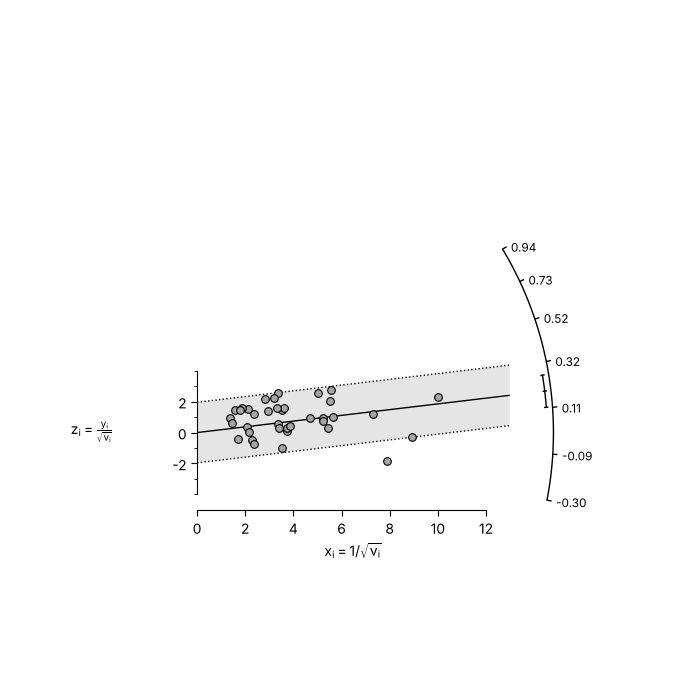
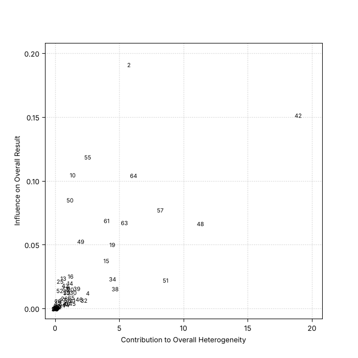
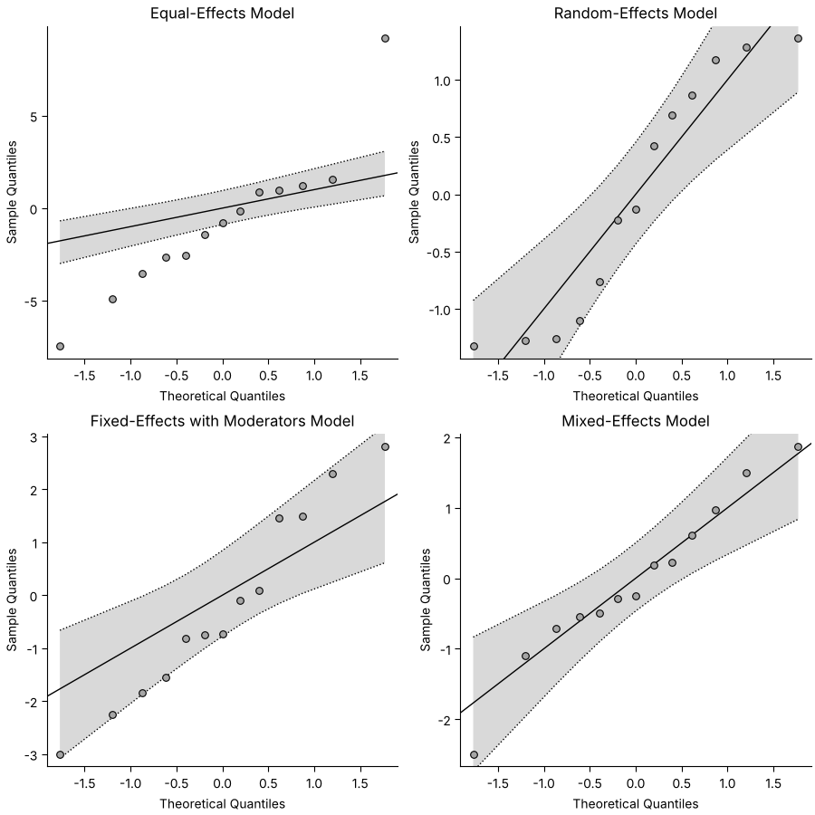
The gallery has more examples of each plot, and the plot of the influence diagnostics, the GOSH plot and the L'Abbe plot.

Interactive charts

metafopy.interactive builds the forest and funnel plots as interactive Altair (Vega-Lite) charts, for notebooks, the web and reports. It needs the interactive extra (see Install) and is not loaded by import metafopy. Hovering a study shows its estimate, interval and weight, and clicking a study highlights it. Both functions take an intercept-only fit and return a chart.

import metafopy.interactive

forest_chart = metafopy.interactive.forest_chart(res, transf=numpy.exp, refline=1.0, xlab='Risk ratio')
funnel_chart = metafopy.interactive.funnel_chart(res)
forest_chart.save('forest.html')
funnel_chart.save('funnel.html')

Function	Chart
forest_chart	Row per study with a square sized by weight, then the pooled estimate as a diamond with its prediction interval; groups and group_fits add a pooled row per subgroup, and href links each study
funnel_chart	Funnel plot with the pseudo-confidence region; a trimfill result draws the imputed studies as open circles
chart_data	The frames behind both charts, as a ChartData, to inspect or build on

The charts inline their data and use fixed colours, so they look the same wherever they are embedded. The showcase notebook links them to other charts.

Styling

Fonts and sizes are matplotlib's. fonts takes the family names metafor uses ('sans', 'serif', 'mono'), and cex, cex_lab, cex_axis scale the text as in R. For anything else, pass your own ax= and use matplotlib on it.