Plot gallery

This page reproduces plots of the plot gallery of the metafor project, with the same datasets and the same models. The figures are drawn by metafopy from the code shown with each of them (Viechtbauer, 2010, https://doi.org/10.18637/jss.v036.i03). For the figures of metafopy next to those of R metafor 5.2-1, see Plots compared with metafor.

The Python code of each figure is run by the test suite, so it cannot rot. The figures are rendered with python bin/gallery.py and Rscript src/tests/r/gallery.R, see Rendering the figures.

import matplotlib

matplotlib.use('Agg')

import math
import matplotlib.colors
import matplotlib.patches
import matplotlib.pyplot
import numpy
import pandas
import scipy.special
import scipy.stats

from metafopy import (
    addpoly,
    baujat,
    cumul,
    datasets,
    escalc,
    forest,
    funnel,
    gosh,
    influence,
    labbe,
    llplot,
    permutest,
    plot_cumul,
    plot_gosh,
    plot_infl,
    plot_permutest,
    plot_vif,
    predict,
    qqnorm,
    radial,
    regplot,
    regtest,
    rma,
    rma_mv,
    set_seed,
    trimfill,
    vcalc,
    vif,
)

matplotlib.rcParams['mathtext.default'] = 'regular'
DPI = 100  # the R figures are rendered at the same size and resolution


def pvalue(p: float) -> str:
    """A p-value as metafor's fmtp2 writes it."""
    if p < 0.001:
        return 'p < .001'
    return f'p = {p:.3f}'.replace('0.', '.') if p < 0.1 else f'p = {p:.2f}'.replace('0.', '.')


def fit_stats(text: str, fit) -> str:
    """The label of a model with its Q-test, I^2 and tau^2 (the helper `mlabfun` of the metafor pages)."""
    return f'{text} (Q = {fit.QE:.2f}, df = {fit.k - fit.p}, {pvalue(fit.QEp)}; $I^2$ = {fit.I2:.1f}%, $\\tau^2$ = {fit.tau2:.2f})'

Forest plots

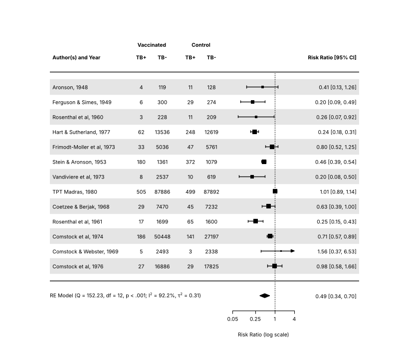
All forest plots of this section use the BCG vaccine data.

dat = escalc(measure='RR', ai='tpos', bi='tneg', ci='cpos', di='cneg', data=datasets.load('dat.bcg'))
dat['slab'] = dat['author'] + ', ' + dat['year'].astype(str)
res = rma('yi', 'vi', data=dat, slab=dat['slab'])
counts = dat[['tpos', 'tneg', 'cpos', 'cneg']].to_numpy()

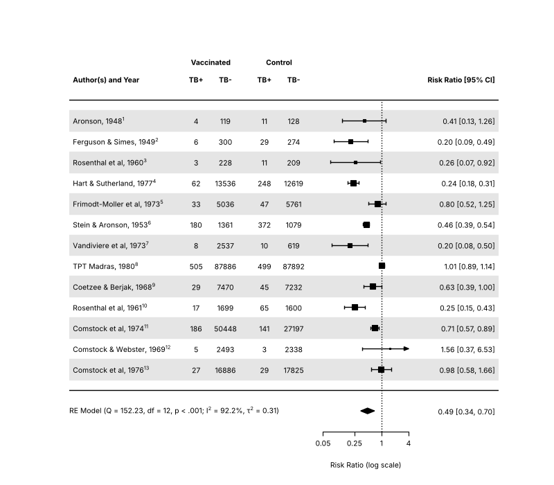
Forest plot with extra annotations

Source: https://www.metafor-project.org/doku.php/plots:forest_plot

fig, ax = matplotlib.pyplot.subplots(figsize=(8, 7))
forest(
    res,
    ax=ax,
    atransf=numpy.exp,
    at=numpy.log([0.05, 0.25, 1, 4]),
    xlim=(-16, 6),
    ilab=counts,
    ilab_lab=['TB+', 'TB-', 'TB+', 'TB-'],
    ilab_xpos=[-9.5, -8, -6, -4.5],
    cex=0.75,
    header='Author(s) and Year',
    mlab='',
    shade=True,
)
ax.text(-8.75, res.k + 2.8, 'Vaccinated', ha='center', va='center', fontsize=7.5, fontweight='bold')
ax.text(-5.25, res.k + 2.8, 'Control', ha='center', va='center', fontsize=7.5, fontweight='bold')
ax.text(-16, -1, fit_stats('RE Model', res), ha='left', va='center', fontsize=7.5)
fig.savefig('forest.png', dpi=DPI)

Forest plot with adjusted text position

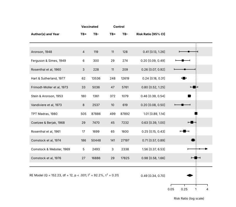
Source: https://www.metafor-project.org/doku.php/plots:forest_plot_with_textpos

fig, ax = matplotlib.pyplot.subplots(figsize=(8, 7))
forest(
    res,
    ax=ax,
    atransf=numpy.exp,
    at=numpy.log([0.05, 0.25, 1, 4]),
    xlim=(-20, 2),
    ilab=counts,
    ilab_lab=['TB+', 'TB-', 'TB+', 'TB-'],
    ilab_xpos=[-13.5, -12, -10, -8.5],
    cex=0.75,
    header='Author(s) and Year',
    mlab='',
    textpos=(-20, -3.5),
    shade=True,
)
ax.text(-12.75, res.k + 2.8, 'Vaccinated', ha='center', va='center', fontsize=7.5, fontweight='bold')
ax.text(-9.25, res.k + 2.8, 'Control', ha='center', va='center', fontsize=7.5, fontweight='bold')
ax.text(-20, -1, fit_stats('RE Model', res), ha='left', va='center', fontsize=7.5)
fig.savefig('forest_textpos.png', dpi=DPI)

Forest plot with subgroups

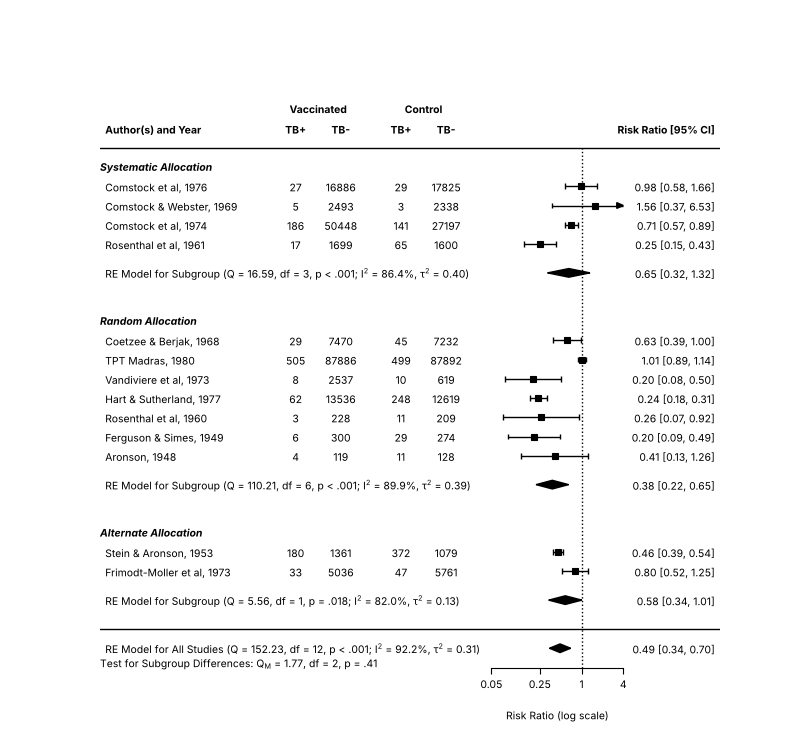
Source: https://www.metafor-project.org/doku.php/plots:forest_plot_with_subgroups

The rows argument places the studies of the three allocation groups, and addpoly adds the summary of each group.

fig, ax = matplotlib.pyplot.subplots(figsize=(8, 7.5))
forest(
    res,
    ax=ax,
    xlim=(-16, 4.6),
    at=numpy.log([0.05, 0.25, 1, 4]),
    atransf=numpy.exp,
    ilab=counts,
    ilab_lab=['TB+', 'TB-', 'TB+', 'TB-'],
    ilab_xpos=[-9.5, -8, -6, -4.5],
    cex=0.75,
    ylim=(-2, 28),
    top=4,
    order=dat['alloc'],
    rows=numpy.r_[3:5, 9:16, 20:24],
    mlab=fit_stats('RE Model for All Studies', res),
    psize=1,
    header='Author(s) and Year',
)
ax.text(-8.75, 27, 'Vaccinated', ha='center', va='center', fontsize=7.5, fontweight='bold')
ax.text(-5.25, 27, 'Control', ha='center', va='center', fontsize=7.5, fontweight='bold')
for y, label in ((24, 'Systematic Allocation'), (16, 'Random Allocation'), (5, 'Alternate Allocation')):
    ax.text(-16, y, label, ha='left', va='center', fontsize=7.5, fontweight='bold', fontstyle='italic')
for name, row in (('systematic', 18.5), ('random', 7.5), ('alternate', 1.5)):
    sub = rma('yi', 'vi', data=dat, subset=(dat['alloc'] == name).to_numpy(), slab=dat['slab'])
    addpoly(sub, ax=ax, row=row, mlab=fit_stats('RE Model for Subgroup', sub))
mods = rma('yi', 'vi', mods='~ alloc', data=dat)
ax.text(-16, -1.8, f'Test for Subgroup Differences: $Q_M$ = {mods.QM:.2f}, df = {mods.p - 1}, {pvalue(mods.QMp)}', ha='left', va='center', fontsize=7.5)
fig.savefig('forest_subgroups.png', dpi=DPI)

Forest plot with multiple CIs

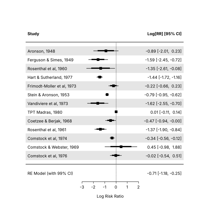
Source: https://www.metafor-project.org/doku.php/plots:forest_plot_with_multiple_cis

The plot shows the 95% CIs of the studies as thin lines and the 80% CIs on top of them as thick lines. forest has no line width argument, so the thick lines are drawn with matplotlib, and the pooled estimate is added with a 99% CI.

fig, ax = matplotlib.pyplot.subplots(figsize=(7, 7))
forest(dat['yi'], dat['vi'], ax=ax, slab=dat['slab'], xlim=(-8, 6), ylim=(-2, len(dat) + 3), psize=1, efac=0, shade=True)
half = scipy.stats.norm.ppf(0.9) * numpy.sqrt(dat['vi'])
ax.hlines(numpy.arange(len(dat), 0, -1), dat['yi'] - half, dat['yi'] + half, color='black', linewidth=3, zorder=5)
addpoly(res, ax=ax, row=-1, level=99, mlab='RE Model (with 99% CI)', annotate=True)
ax.axhline(0, color='black', linewidth=1)
fig.savefig('forest_multiple_cis.png', dpi=DPI)

Forest plot with superscripts

Source: https://www.metafor-project.org/doku.php/plots:forest_plot_with_superscripts

The trial numbers are added to the study labels as superscripts, which some journals require. R writes the labels as plotmath expressions; in matplotlib they are strings with a mathtext part, $^{...}$.

slab_ref = [f'{s}$^{{{t}}}$' for s, t in zip(dat['slab'], dat['trial'])]
fig, ax = matplotlib.pyplot.subplots(figsize=(8, 7))
forest(
    res,
    ax=ax,
    atransf=numpy.exp,
    at=numpy.log([0.05, 0.25, 1, 4]),
    xlim=(-16, 6),
    ilab=counts,
    ilab_lab=['TB+', 'TB-', 'TB+', 'TB-'],
    ilab_xpos=[-9.5, -8, -6, -4.5],
    cex=0.75,
    header='Author(s) and Year',
    mlab='',
    slab=slab_ref,
    shade=True,
)
ax.text(-8.75, res.k + 2.8, 'Vaccinated', ha='center', va='center', fontsize=7.5, fontweight='bold')
ax.text(-5.25, res.k + 2.8, 'Control', ha='center', va='center', fontsize=7.5, fontweight='bold')
ax.text(-16, -1, fit_stats('RE Model', res), ha='left', va='center', fontsize=7.5)
fig.savefig('forest_superscripts.png', dpi=DPI)

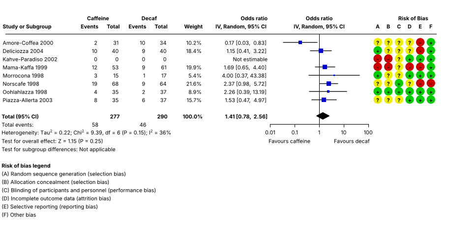
Forest plot in RevMan style

Source: https://www.metafor-project.org/doku.php/plots:forest_plot_revman

The plot mimics the forest plots of RevMan, the software of the Cochrane Collaboration: the counts, the weights and the risk of bias ratings of the studies next to the odds ratios. The study with no events in either group has a missing log odds ratio (drop00=True); na_action='pass' in forest keeps it in the plot (R: options(na.action='na.pass')). R's par(mar=...) becomes subplots_adjust, and the text that forest does not draw is added in data coordinates.

FONT = 10  # R's default text size at cex = 1, in points


def put(ax, x, y, s, pos=None, size=1.0, bold=False, offset=0.5, **kw):
    """R's text(): pos 2 puts the text to the left of x and pos 4 to the right, with an offset of half a character."""
    ha = {None: 'center', 2: 'right', 4: 'left'}[pos]
    dx = {None: 0.0, 2: -1.0, 4: 1.0}[pos] * offset * size * FONT * 0.6
    return ax.annotate(
        s,
        (x, y),
        xytext=(dx, 0),
        textcoords='offset points',
        ha=ha,
        va='center_baseline',
        fontsize=size * FONT,
        fontweight='bold' if bold else 'normal',
        annotation_clip=False,
        **kw,
    )


dat_r = pandas.DataFrame(
    {
        'author': ['Amore-Coffea', 'Deliciozza', 'Kahve-Paradiso', 'Mama-Kaffa', 'Morrocona', 'Norscafe', 'Oohlahlazza', 'Piazza-Allerta'],
        'year': [2000, 2004, 2002, 1999, 1998, 1998, 1998, 2003],
        'ai': [2, 10, 0, 12, 3, 19, 4, 8],
        'n1i': [31, 40, 0, 53, 15, 68, 35, 35],
        'ci': [10, 9, 0, 9, 1, 9, 2, 6],
        'n2i': [34, 40, 0, 61, 17, 64, 37, 37],
    }
)
# the risk of bias of items A to F: + is low, - is high and ? is unclear
bias = {'A': '?+--+?+?', 'B': '??--??+?', 'C': '?????++?', 'D': '??+-+?++', 'E': '--+-+-++', 'F': '+++++-++'}
dat_r = escalc(measure='OR', ai='ai', n1i='n1i', ci='ci', n2i='n2i', data=dat_r, drop00=True)
dat_r['slab'] = dat_r['author'] + ' ' + dat_r['year'].astype(str)
res_r = rma('yi', 'vi', data=dat_r, method='DL', slab=dat_r['slab'])
pred_r = predict(res_r, transf=numpy.exp)
k = len(dat_r)
weights_r = [''] * k
for i, w in zip(numpy.flatnonzero(res_r.data.keep), res_r.weights_()):
    weights_r[i] = f'{w:.1f}%'

fig = matplotlib.pyplot.figure(figsize=(9.13, 4.71))
ax = fig.add_axes((0, 2.18 / 4.71, 1 - 0.26 / 9.13, 1 - 2.18 / 4.71 - 0.36 / 4.71))
sav = forest(
    res_r,
    ax=ax,
    na_action='pass',
    atransf=numpy.exp,
    at=numpy.log([0.01, 0.10, 1, 10, 100]),
    xlim=(-30, 11),
    xlab='',
    efac=(0, 4),
    textpos=(-30, -4.7),
    lty=('solid', 'solid', 'none'),
    refline=None,
    ilab=numpy.column_stack([dat_r['ai'], dat_r['n1i'], dat_r['ci'], dat_r['n2i'], weights_r]),
    ilab_xpos=[-20.6, -18.6, -16.1, -14.1, -10.8],
    ilab_pos=2,
    cex=0.78,
    header=['Study or Subgroup', 'IV, Random, 95% CI'],
    mlab='',
    colout='#0000cc',
    colci='black',
)
x0, x1 = sav.xlim
ixp = sav.ilab_xpos
cx = sav.cex
ax.plot([x0 + 0.5, x1], [k + 1, k + 1], color='black', linewidth=0.8, clip_on=False)
ax.plot([0, 0], [-2, k + 1], color='black', linewidth=0.8, clip_on=False)

for x, s in zip(ixp, ['Events', 'Total', 'Events', 'Total', 'Weight']):
    put(ax, x, k + 2, s, 2, cx, True)
put(ax, (ixp[0] + ixp[1]) / 2, k + 3, 'Caffeine', 2, cx, True)
put(ax, (ixp[2] + ixp[3]) / 2, k + 3, 'Decaf', 2, cx, True)
put(ax, sav.textpos[1], k + 3, 'Odds ratio', 2, cx, True)
put(ax, 0, k + 3, 'Odds ratio', None, cx, True)
put(ax, x1 - 0.6, k + 3, 'Risk of Bias', 2, cx, True)
put(ax, 0, k + 2, 'IV, Random, 95% CI', None, cx, True)
for x, s, pos in [(x0, 'Total (95% CI)', 4), (ixp[1], str(dat_r['n1i'].sum()), 2), (ixp[3], str(dat_r['n2i'].sum()), 2), (ixp[4], '100.0%', 2)]:
    put(ax, x, -1, s, pos, cx, True)
put(ax, x0, -7, 'Risk of bias legend', 4, cx, True)

# hide the summary estimate of forest and add it back in bold
ax.add_patch(matplotlib.patches.Rectangle((sav.textpos[1], -1.5), ixp[4] - sav.textpos[1], 1, facecolor='white', edgecolor='none', zorder=4))
pe, lo, hi = pred_r.pred[0], pred_r.ci_lb[0], pred_r.ci_ub[0]
put(ax, sav.textpos[1], -1, f'{pe:.2f} [{lo:.2f},  {hi:.2f}]', 2, cx, True, zorder=5)

put(ax, math.log(0.01), -4, 'Favours caffeine', 4, cx, offset=-0.5)
put(ax, math.log(100), -4, 'Favours decaf', 2, cx, offset=-0.5)
put(ax, sav.textpos[1], k + 1 - (numpy.flatnonzero(numpy.isnan(dat_r['yi'])) + 1)[0], 'Not estimable', 2, cx)
put(ax, x0, -2, 'Total events:', 4, cx)
put(ax, ixp[0], -2, str(dat_r['ai'].sum()), 2, cx)
put(ax, ixp[2], -2, str(dat_r['ci'].sum()), 2, cx)
put(
    ax,
    x0,
    -3,
    f'Heterogeneity: Tau$^2$ = {res_r.tau2:.2f}; Chi$^2$ = {res_r.QE:.2f}, df = {res_r.k - res_r.p} (P = {res_r.QEp:.2f}); $I^2$ = {round(res_r.I2)}%',
    4,
    cx,
)
put(ax, x0, -4, f'Test for overall effect: Z = {res_r.zval[0]:.2f} (P = {res_r.pval[0]:.2f})', 4, cx)
put(ax, x0, -5, 'Test for subgroup differences: Not applicable', 4, cx)

colors = {'+': '#00cc00', '-': '#cc0000', '?': '#eeee00'}
for letter, xp in zip('ABCDEF', numpy.linspace(x1 - 5.5, x1 - 0.5, 6)):
    ax.scatter([xp] * k, numpy.arange(k, 0, -1), s=130, color=[colors[c] for c in bias[letter]], clip_on=False, zorder=3)
    for y, c in zip(range(k, 0, -1), bias[letter]):
        put(ax, xp, y, c, None, cx, True, zorder=4)
    put(ax, xp, k + 2, letter, None, cx, True)
for y, s in zip(
    range(-8, -14, -1),
    [
        '(A) Random sequence generation (selection bias)',
        '(B) Allocation concealment (selection bias)',
        '(C) Blinding of participants and personnel (performance bias)',
        '(D) Incomplete outcome data (attrition bias)',
        '(E) Selective reporting (reporting bias)',
        '(F) Other bias',
    ],
):
    put(ax, x0, y, s, 4, cx)
fig.savefig('forest_revman.png', dpi=DPI)

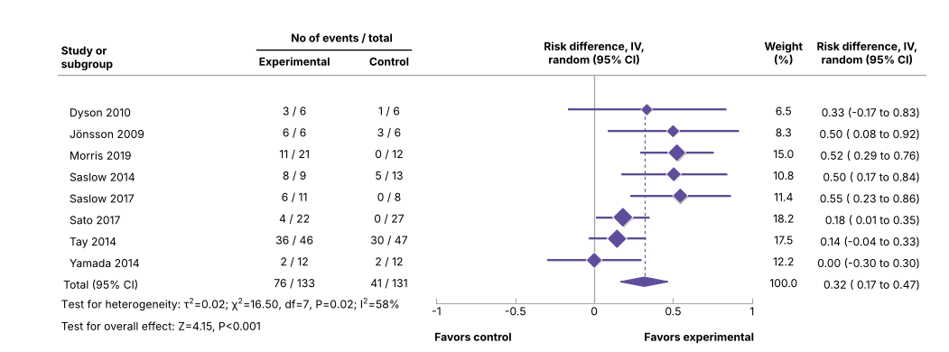
Forest plot in BMJ style

Source: https://www.metafor-project.org/doku.php/plots:forest_plot_bmj

The plot mimics the forest plots of the BMJ, for the risk differences of the studies of Goldenberg et al. (2021), https://doi.org/10.1136/bmj.m4743: the studies are drawn as diamonds sized by their weights, with the CI lines, the vertical reference lines and the summary polygon in the colours of the journal. The CI lines and markers are drawn again on top of those of forest, as in R. (put is the helper of the RevMan plot above.)

dat_b = pandas.DataFrame(
    {
        'author': ['Dyson', 'Jönsson', 'Morris', 'Saslow', 'Saslow', 'Sato', 'Tay', 'Yamada'],
        'year': [2010, 2009, 2019, 2014, 2017, 2017, 2014, 2014],
        'ai': [3, 6, 11, 8, 6, 4, 36, 2],
        'n1i': [6, 6, 21, 9, 11, 22, 46, 12],
        'ci': [1, 3, 0, 5, 0, 0, 30, 2],
        'n2i': [6, 6, 12, 13, 8, 27, 47, 12],
    }
)
dat_b = escalc(measure='RD', ai='ai', n1i='n1i', ci='ci', n2i='n2i', data=dat_b, addyi=False)
dat_b['slab'] = '  ' + dat_b['author'] + ' ' + dat_b['year'].astype(str)
res_b = rma('yi', 'vi', data=dat_b, method='DL', slab=dat_b['slab'])
colp, coll = '#5f4c9a', '#a7a9ac'
k = len(dat_b)
wts = res_b.weights_()
psize = 1.2 + (wts - wts.min()) / (wts.max() - wts.min())
rows = numpy.arange(k, 0, -1)
half = scipy.stats.norm.ppf(0.975) * numpy.sqrt(dat_b['vi'])

fig = matplotlib.pyplot.figure(figsize=(10.51, 3.9))
ax = fig.add_axes((3.2 / 10.51 * 0.2, 2.7 / 3.9 * 0.2, 1 - 1.3 / 10.51 * 0.2 - 3.2 / 10.51 * 0.2, 1 - 2.5 / 3.9 * 0.2 - 2.7 / 3.9 * 0.2))
sav = forest(
    dat_b['yi'],
    dat_b['vi'],
    ax=ax,
    xlim=(-3.4, 2.1),
    ylim=(-1, k + 3),
    alim=(-1, 1),
    cex=0.88,
    header=False,
    pch=18,
    psize=psize,
    efac=0,
    refline=None,
    lty=('solid', 'none'),
    xlab='',
    slab=dat_b['slab'],
    ilab=numpy.column_stack(
        [dat_b['ai'].astype(str) + ' / ' + dat_b['n1i'].astype(str), dat_b['ci'].astype(str) + ' / ' + dat_b['n2i'].astype(str), [f'{w:.1f}' for w in wts]]
    ),
    ilab_xpos=[-1.9, -1.3, 1.2],
    annosym=(' (', ' to ', ')'),
    rowadj=-0.07,
)
x0, x1 = sav.xlim
ixp = sav.ilab_xpos
cx = sav.cex
ax.plot([0, 0], [-1, k + 1.6], color=coll, linewidth=1, clip_on=False)
ax.plot([res_b.beta[0]] * 2, [0, k], color=colp, linewidth=0.8, linestyle=(0, (3, 3)))
ax.hlines(rows, dat_b['yi'] - half, dat_b['yi'] + half, color=colp, linewidth=1.5, zorder=3)
ax.scatter(dat_b['yi'], rows, marker='D', s=(psize * 1.15 * 6.3) ** 2 / 2, color='white', zorder=4)
ax.scatter(dat_b['yi'], rows, marker='D', s=(psize * 6.3) ** 2 / 2, color=colp, zorder=5)
addpoly(res_b, ax=ax, row=0, mlab='Total (95% CI)', efac=2, col=colp, border=colp)
ax.plot([x0, x1], [k + 1.6] * 2, color=coll, linewidth=1, clip_on=False)
ax.spines['bottom'].set_color(coll)
ax.tick_params(axis='x', color=coll, direction='in', pad=1)

put(ax, x0, k + 2.5, 'Study or\nsubgroup', 4, cx, True, offset=0.5)
put(ax, ixp[0], k + 2.3, 'Experimental', None, cx, True)
put(ax, ixp[1], k + 2.3, 'Control', None, cx, True)
put(ax, (ixp[0] + ixp[1]) / 2, k + 3.4, 'No of events / total', None, cx, True)
put(ax, 0, k + 2.7, 'Risk difference, IV,\nrandom (95% CI)', None, cx, True)
ax.plot([ixp[0] - 0.24, ixp[1] + 0.14], [k + 2.8] * 2, color='black', linewidth=1, clip_on=False)
put(ax, ixp[2], k + 2.7, 'Weight\n(%)', None, cx, True)
put(ax, x1 - 0.37, k + 2.7, 'Risk difference, IV,\nrandom (95% CI)', None, cx, True)
put(ax, -1, -2.5, 'Favors control', 4, cx, True, offset=-0.3)
put(ax, 1, -2.5, 'Favors experimental', 2, cx, True, offset=-0.3)
put(ax, ixp[2], 0, '100.0', None, cx)
put(ax, ixp[0], 0, f'{dat_b["ai"].sum()} / {dat_b["n1i"].sum()}', None, cx)
put(ax, ixp[1], 0, f'{dat_b["ci"].sum()} / {dat_b["n2i"].sum()}', None, cx)
put(
    ax,
    x0,
    -1,
    f'Test for heterogeneity: $\\tau^2$={res_b.tau2:.2f}; $\\chi^2$={res_b.QE:.2f}, df={res_b.k - res_b.p}, P={res_b.QEp:.2f}; $I^2$={round(res_b.I2)}%',
    4,
    cx,
)
put(ax, x0, -2, f'Test for overall effect: Z={res_b.zval[0]:.2f}, P<0.001', 4, cx)
fig.savefig('forest_bmj.png', dpi=DPI)

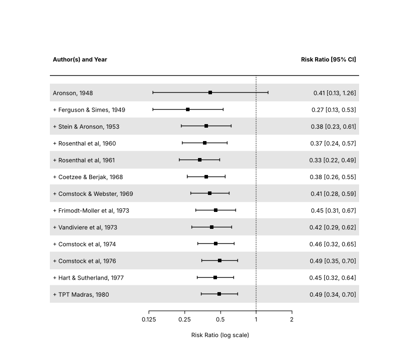
Cumulative forest plot

Source: https://www.metafor-project.org/doku.php/plots:cumulative_forest_plot

tmp = cumul(res, order='year')
fig, ax = matplotlib.pyplot.subplots(figsize=(8, 7))
forest(
    tmp,
    ax=ax,
    xlim=(-4, 2),
    at=numpy.log([0.125, 0.25, 0.5, 1, 2]),
    shade=True,
    atransf=numpy.exp,
    digits=(2, 3),
    cex=0.85,
    header='Author(s) and Year',
)
fig.savefig('forest_cumul.png', dpi=DPI)

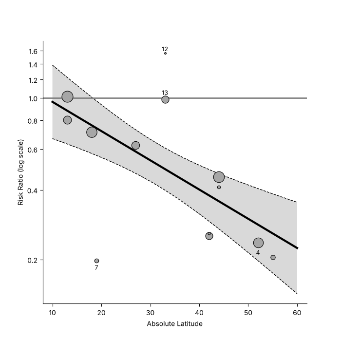
Meta-analytic scatterplot

Source: https://www.metafor-project.org/doku.php/plots:meta_analytic_scatterplot

res_m = rma('yi', 'vi', mods='~ ablat', data=dat)
fig, ax = matplotlib.pyplot.subplots(figsize=(7, 7))
regplot(
    res_m,
    ax=ax,
    xlim=(10, 60),
    predlim=(10, 60),
    xlab='Absolute Latitude',
    refline=0,
    atransf=numpy.exp,
    at=numpy.log(numpy.arange(0.2, 1.61, 0.2)),
    digits=1,
    label=[3, 6, 11, 12],
    offset=(1.6, 0.8),
    labsize=0.9,
    las=1,
    bty='l',
)
fig.savefig('regplot.png', dpi=DPI)

Funnel plots

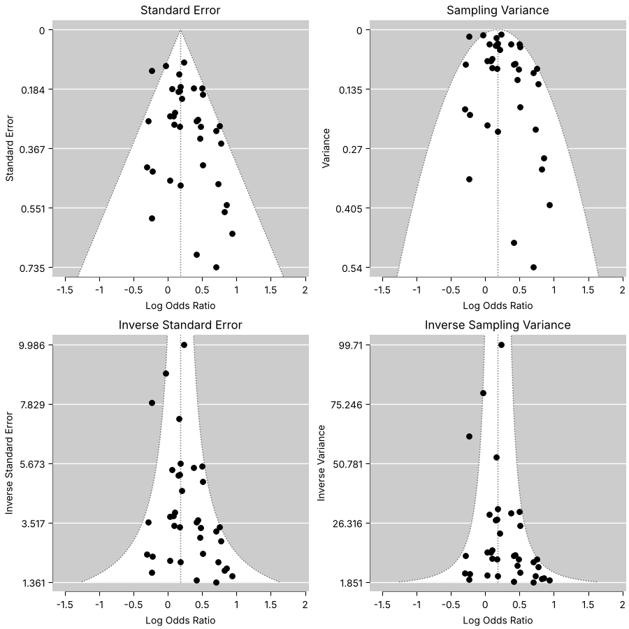
Funnel plot variations

Source: https://www.metafor-project.org/doku.php/plots:funnel_plot_variations

res_h = rma('yi', 'vi', data=datasets.load('dat.hackshaw1998'), measure='OR', method='EE')
fig, axes = matplotlib.pyplot.subplots(2, 2, figsize=(9, 9), layout='constrained')
funnel(res_h, ax=axes[0, 0])
axes[0, 0].set_title('Standard Error')
funnel(res_h, yaxis='vi', ax=axes[0, 1])
axes[0, 1].set_title('Sampling Variance')
funnel(res_h, yaxis='seinv', ax=axes[1, 0])
axes[1, 0].set_title('Inverse Standard Error')
funnel(res_h, yaxis='vinv', ax=axes[1, 1])
axes[1, 1].set_title('Inverse Sampling Variance')
fig.savefig('funnel_variations.png', dpi=DPI)

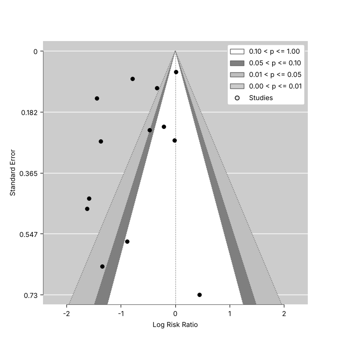
Contour-enhanced funnel plot

Source: https://www.metafor-project.org/doku.php/plots:contour_enhanced_funnel_plot

Contour-enhanced funnel plots (Peters et al., 2008, https://doi.org/10.1016/j.jclinepi.2007.11.010) shade the regions of statistical significance.

res_b = rma(measure='RR', ai='tpos', bi='tneg', ci='cpos', di='cneg', data=datasets.load('dat.bcg'))
fig, ax = matplotlib.pyplot.subplots(figsize=(7, 7))
funnel(res_b, ax=ax, level=[90, 95, 99], refline=0, legend=True)
fig.savefig('funnel_contour.png', dpi=DPI)

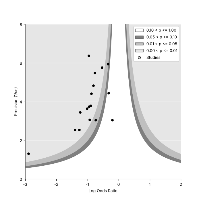
Contour-enhanced funnel plot with the precision on the vertical axis

Source: https://www.metafor-project.org/doku.php/plots:contour_enhanced_funnel_plot_2

dat_g = escalc(measure='OR', ai='ai', n1i='n1i', ci='ci', n2i='n2i', data=datasets.load('dat.graves2010'))
fig, ax = matplotlib.pyplot.subplots(figsize=(7, 7))
funnel(
    dat_g['yi'],
    dat_g['vi'],
    ax=ax,
    yaxis='seinv',
    ylab='Precision (1/se)',
    xlim=(-3, 2),
    ylim=(0.00001, 8),
    level=[0.10, 0.05, 0.01],
    legend=True,
    back='gray90',
    lty=0,
)
ax.set_xlim(-3, 2)
ax.set_ylim(0.00001, 8)
fig.savefig('funnel_contour2.png', dpi=DPI)

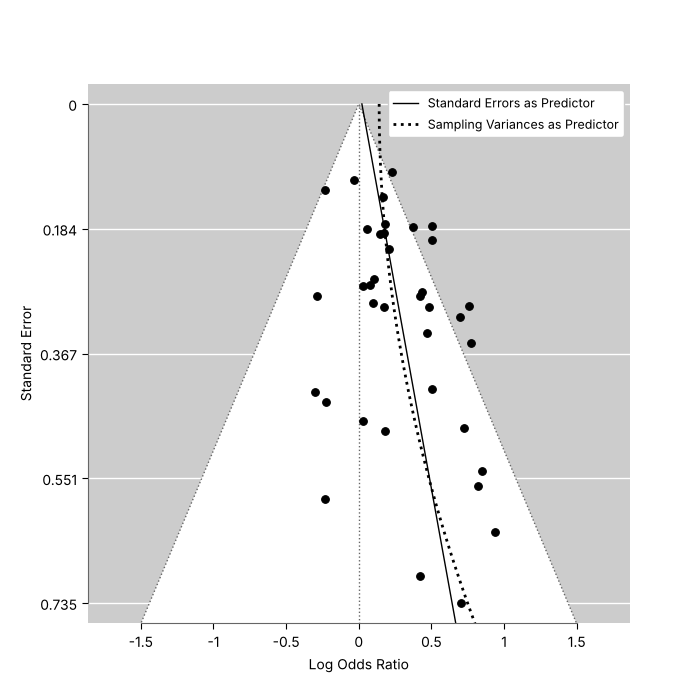
Funnel plot with limit estimate

Source: https://www.metafor-project.org/doku.php/plots:funnel_plot_with_limit_estimate

The regression lines of the regression test for funnel plot asymmetry (regtest, Egger et al., 1997, https://doi.org/10.1136/bmj.315.7109.629) are added with matplotlib.

res_l = rma('yi', 'vi', data=datasets.load('dat.hackshaw1998'), measure='OR')
fig, ax = matplotlib.pyplot.subplots(figsize=(7, 7))
funnel(res_l, ax=ax, refline=0)
se = numpy.linspace(0, 0.8, 100)
reg = regtest(res_l, ret_fit=True)
ax.plot(reg.fit.beta[0] + reg.fit.beta[1] * se, se, color='black', linewidth=1, label='Standard Errors as Predictor')
reg = regtest(res_l, predictor='vi', ret_fit=True)
ax.plot(reg.fit.beta[0] + reg.fit.beta[1] * se**2, se, color='black', linewidth=2, linestyle=':', label='Sampling Variances as Predictor')
ax.legend(loc='upper right', fontsize=9, framealpha=1)
fig.savefig('funnel_limit.png', dpi=DPI)

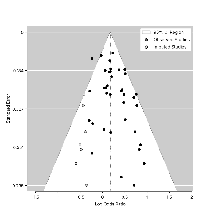
Funnel plot with trim and fill

Source: https://www.metafor-project.org/doku.php/plots:funnel_plot_with_trim_and_fill

taf = trimfill(rma('yi', 'vi', data=datasets.load('dat.hackshaw1998'), measure='OR'))
fig, ax = matplotlib.pyplot.subplots(figsize=(7, 7))
funnel(taf, ax=ax, legend={'show': 'cis'})
fig.savefig('funnel_trimfill.png', dpi=DPI)

Other plots

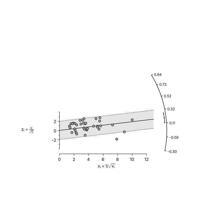
Radial plot

Source: https://www.metafor-project.org/doku.php/plots:radial_plot

res_r = rma('yi', 'vi', data=datasets.load('dat.hackshaw1998'), method='EE')
fig, ax = matplotlib.pyplot.subplots(figsize=(7, 7))
radial(res_r, ax=ax)
fig.savefig('radial.png', dpi=DPI)

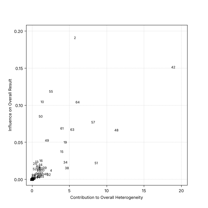
Baujat plot

Source: https://www.metafor-project.org/doku.php/plots:baujat_plot

dat_p = datasets.load('dat.pignon2000')
dat_p['yi'] = dat_p['OmE'] / dat_p['V']
dat_p['vi'] = 1 / dat_p['V']
res_p = rma('yi', 'vi', data=dat_p, method='EE', slab=dat_p['id'])
fig, ax = matplotlib.pyplot.subplots(figsize=(7, 7))
baujat(res_p, ax=ax, xlim=(0, 20), ylim=(0, 0.2))
fig.savefig('baujat.png', dpi=DPI)

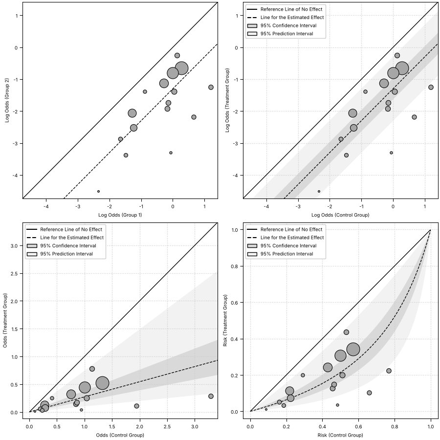
L'Abbe plots

Source: https://www.metafor-project.org/doku.php/plots:labbe_plot

dat_d = datasets.load('dat.damico2009')
res_d = rma(measure='OR', ai='xt', n1i='nt', ci='xc', n2i='nc', data=dat_d)
cells = {'ai': dat_d['xt'], 'bi': dat_d['nt'] - dat_d['xt'], 'ci_counts': dat_d['xc'], 'di': dat_d['nc'] - dat_d['xc']}
fig, axes = matplotlib.pyplot.subplots(2, 2, figsize=(9, 9), layout='constrained')
with matplotlib.rc_context({'font.size': 7}):  # R's par(cex=0.7)
    labbe(res_d, **cells, ax=axes[0, 0])
    labbe(res_d, **cells, ci=True, pi=True, grid=True, legend=True, xlab='Log Odds (Control Group)', ylab='Log Odds (Treatment Group)', ax=axes[0, 1])
    labbe(res_d, **cells, ci=True, pi=True, grid=True, legend=True, transf=numpy.exp, xlab='Odds (Control Group)', ylab='Odds (Treatment Group)', ax=axes[1, 0])
    labbe(
        res_d,
        **cells,
        ci=True,
        pi=True,
        grid=True,
        legend=True,
        transf=scipy.special.expit,
        lim=(0, 1),
        xlab='Risk (Control Group)',
        ylab='Risk (Treatment Group)',
        ax=axes[1, 1],
    )
fig.savefig('labbe.png', dpi=DPI)

Normal quantile-quantile plots

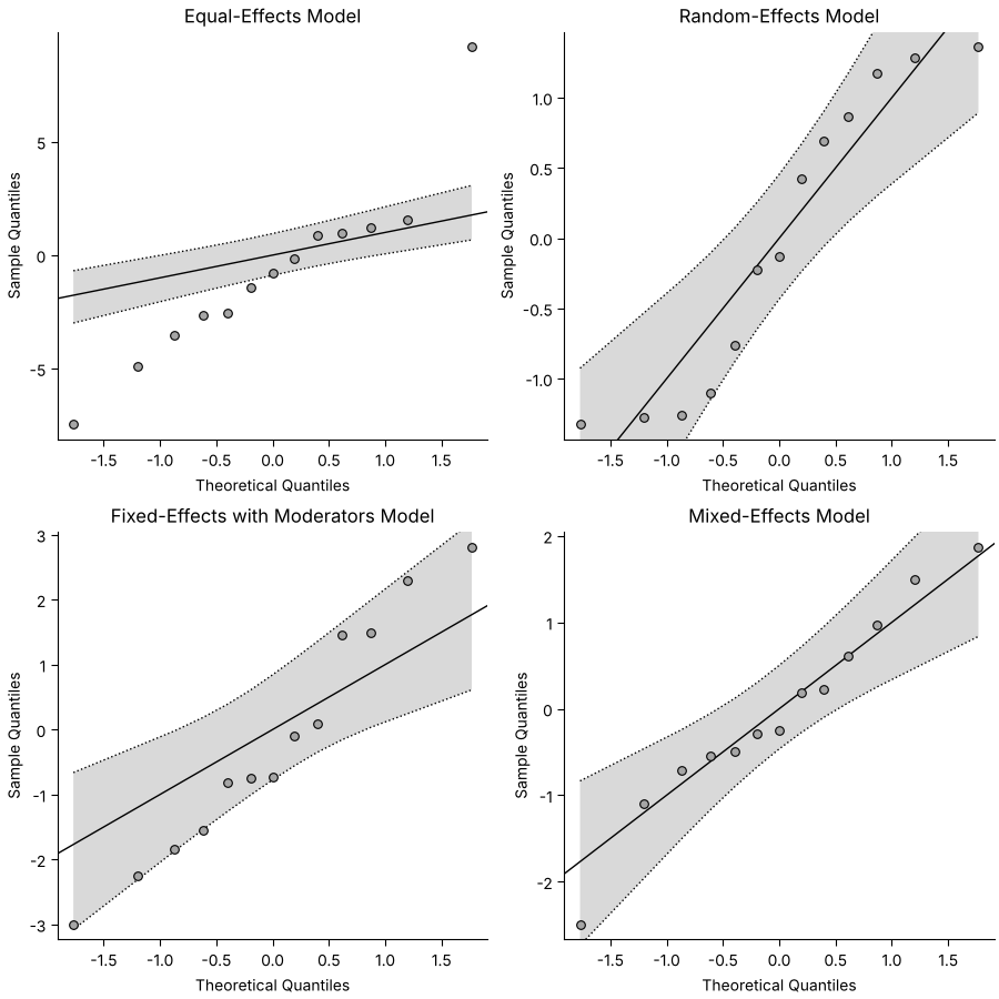
Source: https://www.metafor-project.org/doku.php/plots:normal_qq_plots

models = {
    'Equal-Effects Model': rma('yi', 'vi', data=dat, method='EE'),
    'Random-Effects Model': rma('yi', 'vi', data=dat),
    'Fixed-Effects with Moderators Model': rma('yi', 'vi', mods='~ ablat', data=dat, method='FE'),
    'Mixed-Effects Model': rma('yi', 'vi', mods='~ ablat', data=dat),
}
fig, axes = matplotlib.pyplot.subplots(2, 2, figsize=(9, 9), layout='constrained')
for ax, (title, fit) in zip(axes.flat, models.items(), strict=True):
    qqnorm(fit, ax=ax, seed=1234)
    ax.set_title(title)
fig.savefig('qqnorm.png', dpi=DPI)

Plot of influence diagnostics

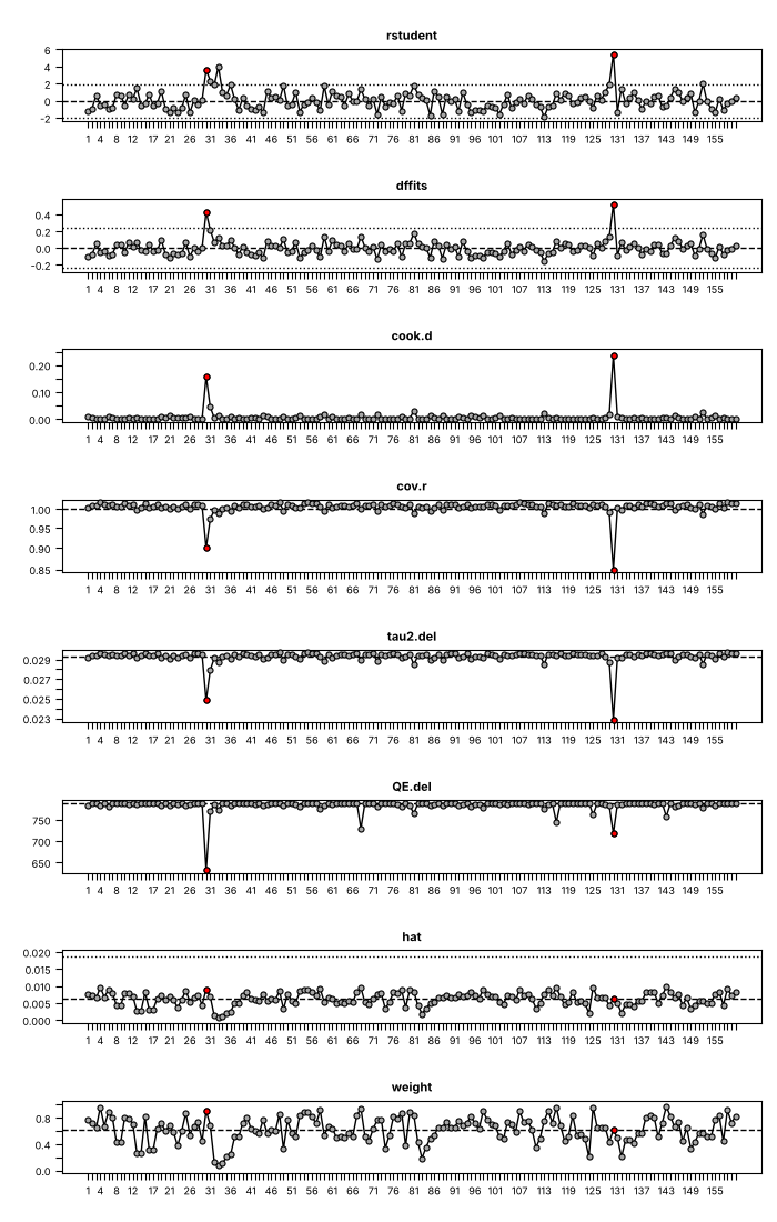
Source: https://www.metafor-project.org/doku.php/plots:plot_of_influence_diagnostics

res_i = rma(ri='ri', ni='ni', measure='ZCOR', data=datasets.load('dat.mcdaniel1994'))
fig, ax = matplotlib.pyplot.subplots(figsize=(7, 11))
ax.set_position((0.08, 0.04, 0.9, 0.92))  # the area the panels fill
plot_infl(influence(res_i), ax=ax, mfrow=(8, 1))
fig.savefig('influence.png', dpi=DPI)

GOSH plot

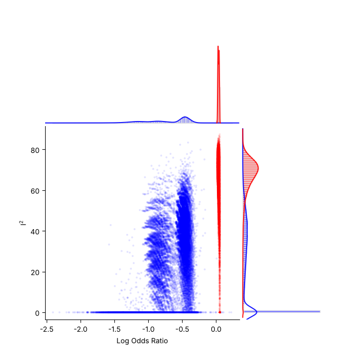
Source: https://www.metafor-project.org/doku.php/plots:gosh_plot

res_e = rma(measure='OR', ai='ai', n1i='n1i', ci='ci', n2i='n2i', data=datasets.load('dat.egger2001'), method='EE')
sav = gosh(res_e)
fig, ax = matplotlib.pyplot.subplots(figsize=(7, 7))
plot_gosh(sav, out=15, breaks=100, ax=ax)
fig.savefig('gosh.png', dpi=DPI)

Plot of cumulative results

Source: https://www.metafor-project.org/doku.php/plots:plot_of_cumulative_results

fig, ax = matplotlib.pyplot.subplots(figsize=(7, 7))
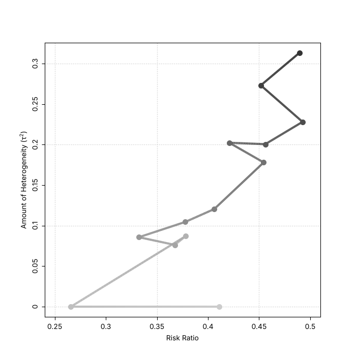
plot_cumul(tmp, ax=ax, transf=numpy.exp, xlim=(0.25, 0.5), lwd=3, cex=1.3)
fig.savefig('cumul.png', dpi=DPI)

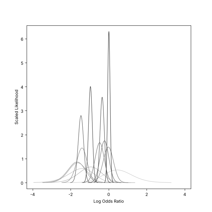
Log-likelihood plot

Source: https://wviechtb.github.io/metafor/reference/llplot.html (an example of the help page of llplot)

fig, ax = matplotlib.pyplot.subplots(figsize=(7, 7))
llplot(measure='OR', ai='tpos', bi='tneg', ci='cpos', di='cneg', data=datasets.load('dat.bcg'), lwd=1, refline=None, xlim=(-4, 4), ax=ax)
fig.savefig('llplot.png', dpi=DPI)

Permutation distributions

Source: https://wviechtb.github.io/metafor/reference/plot.permutest.rma.uni.html (the help page of plot.permutest.rma.uni)

res_p = rma('yi', 'vi', mods='~ ablat + year', data=dat)
set_seed(1234)
perm = permutest(res_p, iter=1000)
fig, ax = matplotlib.pyplot.subplots(figsize=(7, 7))
plot_permutest(perm, QM=True, lwd=(2, 1, 1, 0), legend=True, ax=ax)
fig.savefig('permutest.png', dpi=DPI)

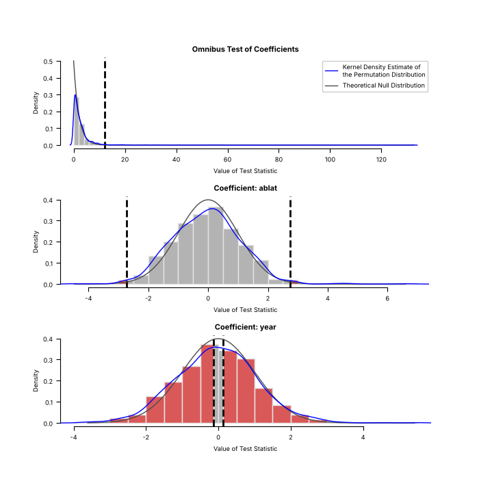
The generator is seeded with set_seed(1234), like R's set.seed(1234), so both figures draw the same permutations and the histograms, axes and densities agree. As in metafor, the legend appears in the first panel only.

Simulated variance inflation factors

Source: https://wviechtb.github.io/metafor/reference/plot.vif.rma.html (the help page of plot.vif.rma)

fig, ax = matplotlib.pyplot.subplots(figsize=(7, 7))
set_seed(1234)
plot_vif(vif(res_p, btt=1, sim=1000, progbar=False), ax=ax)
fig.savefig('vif.png', dpi=DPI)

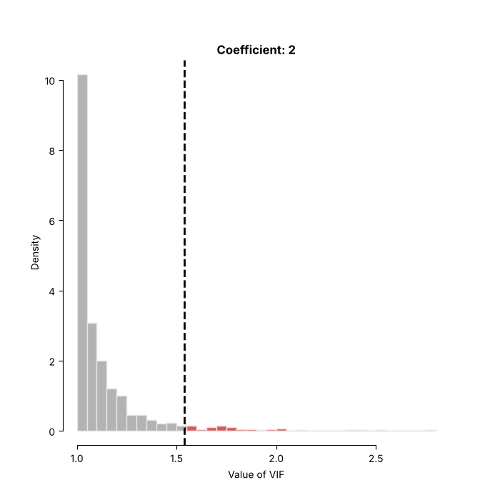
The generator is seeded with set_seed(1234), like R's set.seed(1234), so both figures show the same 1000 simulated values.

Plots of multilevel models

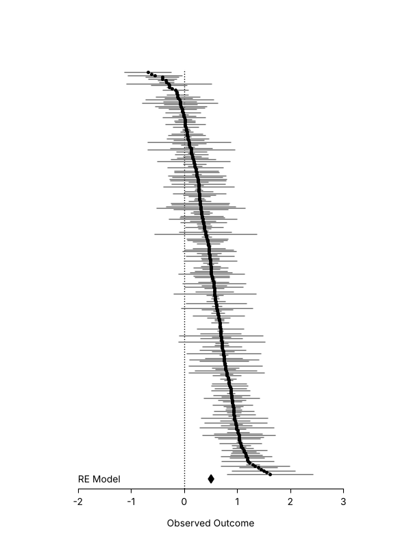
Caterpillar plot

Source: https://www.metafor-project.org/doku.php/plots:caterpillar_plot

The data are simulated as on the metafor page, but with the random number generator of NumPy, so the points are not those of the R figure.

rng = numpy.random.default_rng(5132)
k = 250
vi = rng.chisquare(1, k) * 0.03
yi = rng.normal(rng.normal(0.5, 0.4, k), numpy.sqrt(vi))
res_c = rma(yi, vi)
fig, ax = matplotlib.pyplot.subplots(figsize=(6, 8))
forest(
    yi,
    vi,
    ax=ax,
    header=False,
    xlim=(-2.5, 3.5),
    ylim=(-8, 254),
    order='obs',
    slab=numpy.nan,
    annotate=False,
    efac=(0, 1),
    pch=19,
    colci='gray40',
    psize=2.5,
    cex_lab=1,
    cex_axis=1,
    lty=['solid', 'blank'],
)
addpoly(res_c, ax=ax, mlab='', cex=1)
ax.text(-2, -2, 'RE Model', ha='left', va='center')
fig.savefig('caterpillar.png', dpi=DPI)

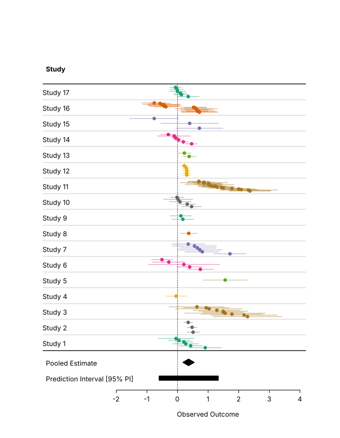
Forest plot with grouped estimates

Source: https://www.metafor-project.org/doku.php/plots:forest_plot_with_grouped_estimates

The effect sizes of a study are drawn on rows close to each other, in a colour per study.

dat_a = datasets.load('dat.assink2016')
V = vcalc(vi=dat_a['vi'], cluster=dat_a['study'], obs=dat_a['esid'], rho=0.6)
res_a = rma_mv(yi='yi', V=V, random='~ 1 | study/esid', data=dat_a)
dat_a = dat_a.sort_values(['study', 'yi'], ascending=False, ignore_index=True)
dat_a['row'] = dat_a['study'].rank(method='dense')
offsets = {1: [0.0], 2: [-0.1, 0.1]}
dat_a['row_seq'] = dat_a['row'] + dat_a.groupby('study')['row'].transform(
    lambda x: pandas.Series(offsets.get(len(x), numpy.linspace(-0.3, 0.3, len(x))), index=x.index)
)
dat_a['slab'] = numpy.where(dat_a['study'].duplicated(), '', 'Study ' + dat_a['study'].astype(str))
palette = matplotlib.colormaps['Dark2'].colors
dat_a['colpt'] = [matplotlib.colors.to_hex(palette[i % len(palette)]) for i in pandas.factorize(dat_a['study'])[0]]
dat_a['colci'] = [matplotlib.colors.to_hex(c, keep_alpha=True)[:7] + '80' for c in dat_a['colpt']]
fig, ax = matplotlib.pyplot.subplots(figsize=(7, 9))
forest(
    dat_a['yi'],
    dat_a['vi'],
    ax=ax,
    rows=dat_a['row_seq'],
    slab=numpy.nan,
    annotate=False,
    xlim=(-4.4, 4.2),
    ylim=(-2.0, dat_a['row'].max() + 2.5),
    cex=1,
    pch=19,
    psize=0.8,
    efac=0,
    col=list(dat_a['colpt']),
    colci=list(dat_a['colci']),
)
for row, label in zip(dat_a['row'], dat_a['slab'], strict=True):
    ax.text(-4.4, row, label, ha='left', va='center_baseline', fontsize=10)
for h in numpy.arange(0, dat_a['row'].max() + 1) + 0.5:
    ax.axhline(h, color='0.2', linewidth=0.2)
addpoly(res_a, ax=ax, row=-0.25, efac=1, mlab='Pooled Estimate', predstyle='bar')
ax.axhline(0.5, color='black', linewidth=1)
fig.savefig('forest_grouped.png', dpi=DPI)

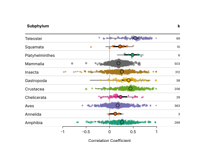
Forest plot in orchard style

Source: https://www.metafor-project.org/doku.php/plots:forest_plot_orchard_style

The correlations of the phylogenetic meta-analysis of Moura et al. (2021) are shown per subphylum, with the points of the studies jittered, and the estimates, CIs and prediction intervals of the model on top.

# docs: skip (the fit takes about a minute and a half; bin/gallery.py runs this block)
dat_m = escalc(measure='ZCOR', ri='ri', ni='ni', data=datasets.load('dat.moura2021'))
levels = sorted(dat_m['subphylum'].unique())
nlvls = len(levels)
res_m = rma_mv('yi', 'vi', mods='~ 0 + subphylum', random=['~ subphylum | study.id', '~ subphylum | effect.size.id'], struct='DIAG', sparse=True, data=dat_m)

# the studies closer to the pooled estimates are jittered more
rng = numpy.random.default_rng(1234)
dat_m['row'] = dat_m['subphylum'].map({name: i + 1 for i, name in enumerate(levels)})
d = numpy.abs(res_m.residuals()) ** (1 / 8)
d = (1 - (d - d.min()) / (d.max() - d.min())) * 0.5
dat_m['row_jitter'] = dat_m['row'] + rng.uniform(-d, d)
palette = matplotlib.colormaps['Dark2'].colors
cols = [matplotlib.colors.to_hex(palette[i % len(palette)]) for i in range(nlvls)]
dat_m['colpt'] = [matplotlib.colors.to_hex(cols[r - 1]) + '99' for r in dat_m['row']]
dat_m['viadj'] = numpy.maximum(dat_m['vi'], dat_m['vi'].quantile(0.05))

fig, ax = matplotlib.pyplot.subplots(figsize=(7, 5))
forest(
    dat_m['yi'],
    dat_m['viadj'],
    ax=ax,
    header='Subphylum',
    rows=dat_m['row_jitter'],
    slab=numpy.nan,
    annotate=False,
    xlim=(-1.8, 1.5),
    ylim=(0.5, nlvls + 2.5),
    cex=1,
    pch=19,
    efac=0,
    col=list(dat_m['colpt']),
    colci='none',
    transf=numpy.tanh,
    digits=1,
    xlab='Correlation Coefficient',
)
for i, name in enumerate(levels, start=1):
    ax.text(-1.8, i, name, ha='left', va='center_baseline', fontsize=10)
for h in numpy.arange(0, nlvls + 1) + 0.5:
    ax.axhline(h, color='0.2', linewidth=0.2)

# points, CIs and PIs of the subphylum levels
pred = predict(res_m, newmods=numpy.eye(res_m.p), tau2_levels=list(range(nlvls)), gamma2_levels=list(range(nlvls)), transf=numpy.tanh)
ypos = numpy.arange(1, nlvls + 1)
ax.hlines(ypos, pred.pi_lb, pred.pi_ub, color='black', linewidth=1)
ax.hlines(ypos, pred.ci_lb, pred.ci_ub, color='black', linewidth=3)
ax.scatter(pred.pred, ypos, s=70, facecolor=cols, edgecolor='black', linewidth=1, zorder=5)
ax.text(1.5, nlvls + 1.5, 'k', ha='right', va='center_baseline', fontsize=10, fontweight='bold')
for i, name in enumerate(levels, start=1):
    ax.text(1.5, i, str((dat_m['subphylum'] == name).sum()), ha='right', va='center_baseline', fontsize=7.5)
fig.savefig('forest_orchard.png', dpi=DPI)

Rendering the figures

The image files are committed under docs/images/gallery. To render them again, from the repository root:

source bin/activate.sh
python bin/gallery.py
LC_ALL=C.UTF-8 Rscript src/tests/r/gallery.R

The first command writes docs/images/gallery/py, the second docs/images/gallery/r (it needs R with metafor 5.2-1 and metadat). The R figures are shown on Plots compared with metafor.